Quick Start Guide

Core Feature

This feature is available in all MATISSE Explorer deployments.

Get started with MATISSE Explorer in just a few minutes. This guide walks you through the essential steps to explore your spatial transcriptomics data.

Step 1: Open Your Project

InSilicoLab Users

If you are using InSilicoLab, select your project from the Reports section to open MATISSE Explorer.

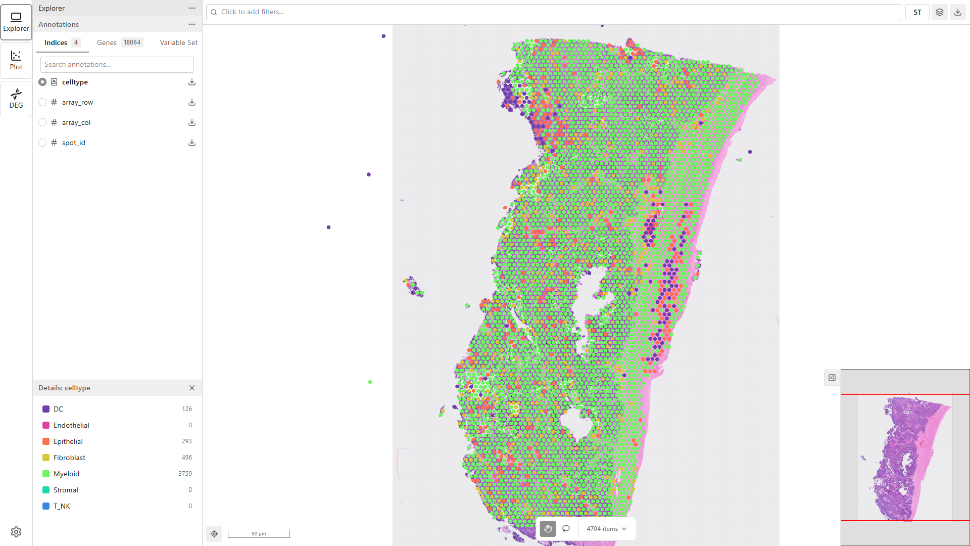
When you launch MATISSE Explorer, your project data loads automatically. You will see:

• The map viewer displaying your tissue image with data points
• The Sidebar showing available annotations
• Loading indicators while data is being fetched

Wait for the data to finish loading before proceeding. Large datasets may take a moment to fully render.

Step 2: Color by Annotation

Apply color mapping to visualize patterns in your data:

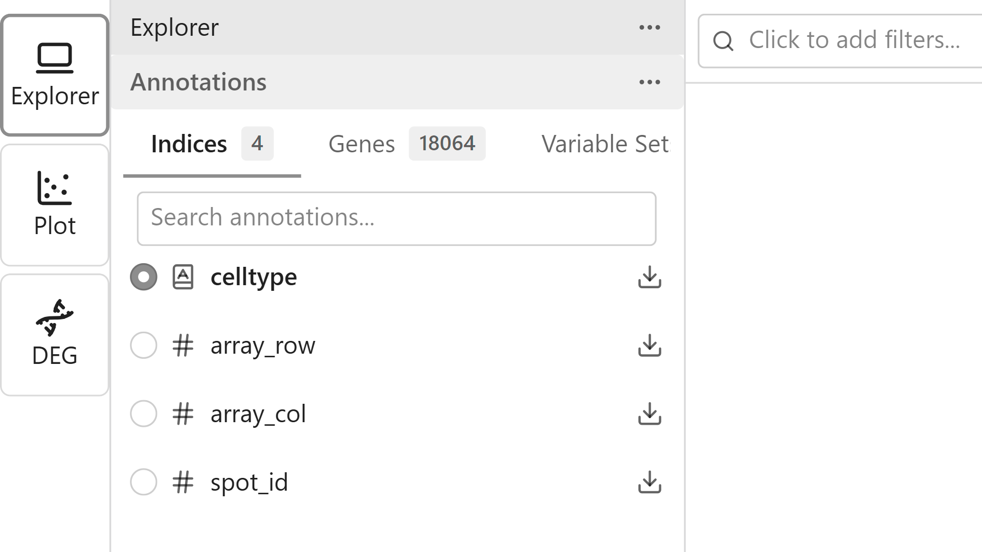
1. In the Sidebar, browse the Annotations list
2. Click the Categorical tab to see cell type annotations
3. Click on an annotation name (e.g., "cell_type") to select it
4. The map updates to show data points colored by the selected annotation

Try Different Annotation Types

• Categorical - Discrete categories like cell types or clusters
• Continuous - Numeric values like gene expression levels
• Embeddings - Dimensionality reduction coordinates

Step 3: Navigate the Map

Explore your data using mouse controls:

Action	Control
Pan	Click and drag
Zoom in	Scroll wheel up or double-click
Zoom out	Scroll wheel down
Reset view	Click the reset/home button in toolbar

Step 4: Apply a Filter

Narrow down your data to specific populations:

1. Click the Filter button in the toolbar to open the Filter Panel
2. Click Add Condition to create a new filter rule
3. Select an annotation and set your criteria
4. The filter applies automatically (Auto apply is enabled by default)

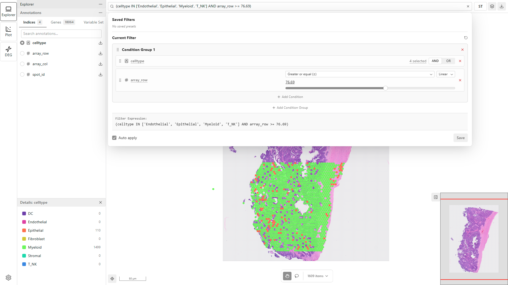
Only data points matching your filter criteria will remain visible. The point count updates to show how many points pass the filter.

Step 5: Use Lasso Selection

Select specific regions interactively:

1. Click the Selection mode button in the toolbar
2. Draw a closed shape around your region of interest
3. Release to complete the selection
4. View the count of selected points

What You Can Do With Selections

• Add the selection as a filter condition
• View statistics for selected points
• Export selected data

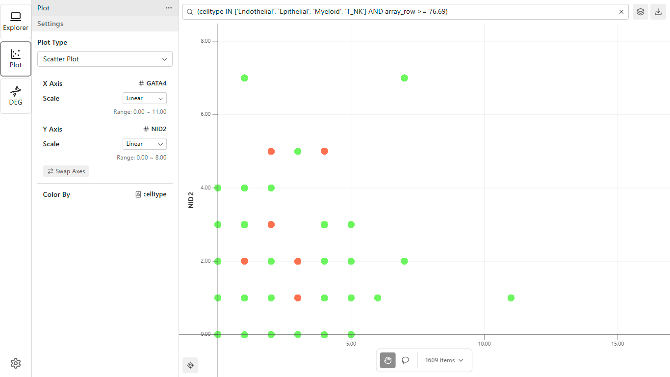
Step 6: View a Scatter Plot

Explore relationships between annotations:

1. Click the Plot icon in the Activity Bar
2. In the Sidebar, configure your X and Y axes
3. Optionally set a color mapping
4. The scatter plot renders in the Workspace

Next Steps

Now that you know the basics, explore more features:

• Map Viewer - Detailed map viewer documentation
• Filter - Build complex filter queries
• Variable Sets - Create custom gene groups
• Tutorials - Step-by-step workflow guides

Tips for New Users

1. Start with categorical annotations - They provide clear visual groupings
2. Use the legend - Hover over legend items to understand the color mapping
3. Save filter presets - Reuse complex filter configurations
4. Try different projections - Switch between spatial, UMAP, and t-SNE views
5. Export early, export often - Save filtered data for downstream analysis