Scatter Plot

Core Feature

This feature is available in all Portrai Explorer deployments.

The Scatter Plot draws each cell or spot as a point positioned by two continuous values — for example two genes, a gene against sequencing depth, or two signature scores. It is the workhorse for inspecting how two measurements relate across a dataset, comparable to a FeatureScatter in Seurat or scanpy.pl.scatter, but interactive: you can pan, zoom, recolor, and lasso-select populations directly on the plot.

Scatter is one of several plot types in the Plot Dashboard. You add it from the dashboard's plot catalog, and it lives as a panel in the grid alongside other plots — so a single scatter plot is no longer the whole workspace. Multiple plots can coexist, and each panel can be renamed, duplicated, resized, dragged, and deleted independently. Per-plot configuration (axes, scales, color, point size) is persisted per project.

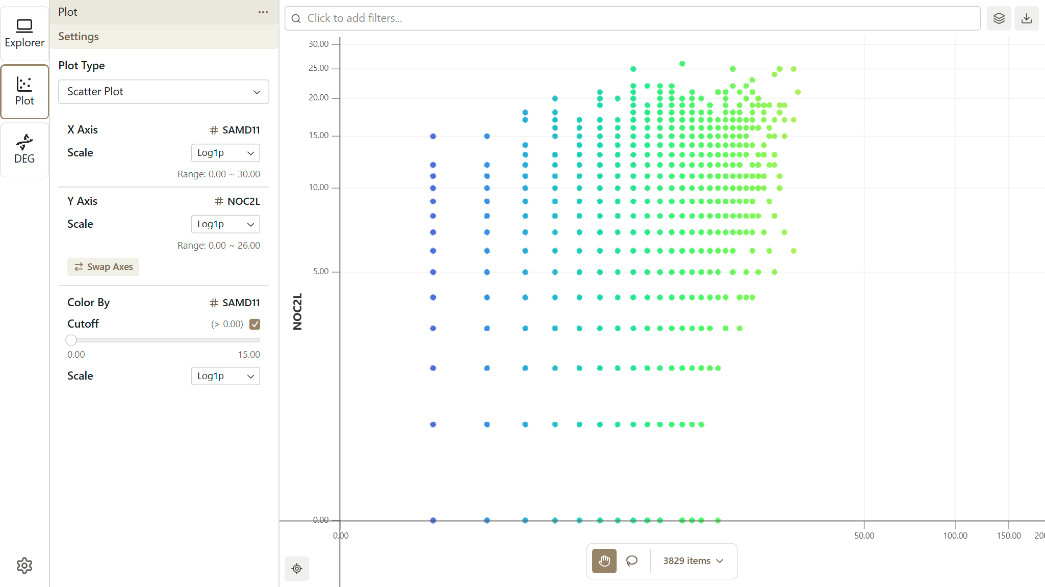
Creating a Scatter Plot

Scatter plots are created from the Plot Dashboard.

1. Open the Plot Dashboard from the Activity Bar.
2. Add a new plot from the catalog and choose Scatter.
3. The new scatter panel appears in the grid, and its configuration options appear in the Sidebar.

The sidebar lists every plot in the dashboard. Selecting a plot makes it the active panel and shows its axis, scale, and color settings. See Plot Dashboard for managing panels (rename, duplicate, resize, delete).

Configuring Axes

X Axis

Select what to display on the horizontal axis:

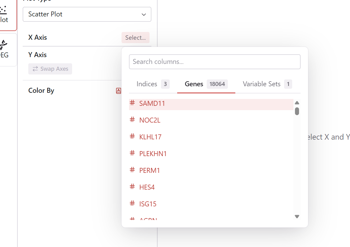
1. Click the X Axis selector
2. Choose from:
   • Continuous features (gene expression, metrics, embedding coordinates)
   • Signature scores
3. The plot updates with the new X axis

TIP

Use the Sort button to organize features alphabetically when browsing long feature lists.

Y Axis

Select what to display on the vertical axis:

1. Click the Y Axis selector
2. Choose from the same options as X axis
3. The plot updates with the new Y axis

Signature Axes

When selecting a Signature for an axis:

1. Choose a Signature from the selector
2. Select a Method to combine variables:

Method	Description
Max	Maximum value among variables
Min	Minimum value among variables
Sum	Sum of variable values
Average	Average of variable values (default)
UMI Count	LogNorm: ln(10000 × sum/totalUMI + 1)

3. Configure the scale type as needed

Swap Axes

Click the Swap Axes button to exchange X and Y axis configurations, including their scale settings.

Common Axis Combinations

X Axis	Y Axis	Purpose
Gene A	Gene B	Compare expression of two genes
Gene	n_counts	Expression vs. sequencing depth
Signature A	Signature B	Compare pathway scores

Scale Types

For each axis, choose an appropriate scale:

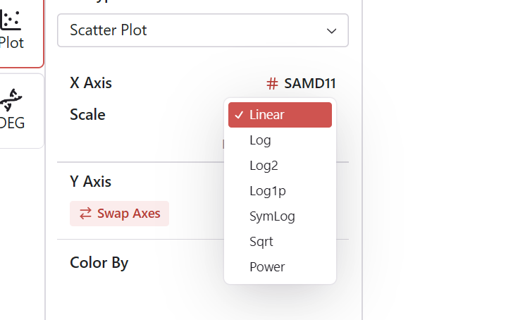
Scale	Best For
Linear	Most data (default)
Log	Wide-ranging positive values
Log2	Wide-ranging positive values (base 2)
Log1p	Data with zeros, single-cell RNA-seq
SymLog	Data with negative values or zeros
Sqrt	Moderate compression
Power	Emphasize differences in small values

TIP

Log and Log2 scales are disabled when the minimum value is negative. Use SymLog or Log1p for data that includes zero or negative values.

Changing Scale

1. Locate the scale selector below each axis configuration
2. Select the desired scale type
3. The plot redraws with the new scaling

Color Mapping

Apply color to points based on feature values:

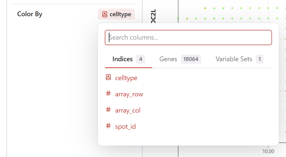
Setting Color

1. Find the Color By selector in the sidebar
2. Choose a feature:
   • Categorical: Points colored by category
   • Continuous: Points colored by value gradient
   • Signature: Points colored by computed score
3. The plot updates with colors

Continuous Color Settings

For continuous features and Signatures, these controls live in the Details Panel (described below), not beside the Color By selector:

• Cutoff: Enable and adjust to filter out low values from the color scale (0-50%)
• Scale: Choose the scale type for color mapping
• Method (Signatures only): Select the combination method

Legend

The legend shows:

• Category names and colors (categorical)
• Color gradient with value range (continuous)

Plot Settings

Open plot settings from the Layers button (layer icon) in the plot panel titlebar — the bar across the top of the panel, beside the ⋯ menu and the ✕ close button. Click it to open the Layer Settings popover.

Draggable Labels

The axis titles and the color legend can be dragged to reposition them on the plot. Once any of these labels has been moved, a Reset label positions button appears in the plot panel titlebar (beside the Layers and Export buttons). Click it to return all labels to their default positions.

Feature Layer

Controls the opacity of all data points:

Control	Description
Opacity slider	0 (transparent) to 1 (opaque)
Eye toggle	Quick show/hide toggle

Point Size

Control	Description
Auto toggle	Enable automatic point sizing
Size slider	Manual size from 1px to 15px

Defaults:

• Auto: Enabled
• Size: 3px (when Auto is disabled)

TIP

Manually adjusting the size slider will automatically disable Auto mode.

Axis Title Size

Adjust the font size of axis titles (10-24px, default 14px).

See Layer Settings for shared point-appearance details.

Details Panel

When the active plot is a Scatter Plot and a color-by is set, the Sidebar shows a Details Panel for the current color-by selection:

• Feature color-by: Displays feature statistics (category counts for categorical, value range for continuous)
• Signature color-by: Displays Signature details including variable list, match status, and combination method controls

The Details Panel updates automatically when you change the color-by setting. It is not shown for other plot types, or when no color-by is set.

Interacting with the Plot

Navigation

Action	Control
Pan	Click and drag
Zoom	Scroll wheel
Reset	Click the reset button (bottom-left)

TIP

Hold the Space key to temporarily switch to Pan mode while in Selection mode.

Hover Information

Hover over points to see:

• Point identifier (Spot ID)
• X axis column name and value
• Y axis column name and value
• Color feature name and value
• Individual variable values (if coloring by Signature)

Lasso Selection on Scatter Plots

Select points directly on the scatter plot using lasso selection.

How to Select

1. Click the Selection button (Lasso icon) in the mode switcher at bottom center
2. Click and drag to draw a closed shape
3. Release to complete selection
4. Selected points are highlighted

Using Plot Selections

Selections made on scatter plots can be:

• Added to the Subset as lasso conditions
• Used to count specific populations
• Combined with other subset conditions

Selection Context

Lasso selections on scatter plots include:

• X axis column name
• Y axis column name
• X and Y scale types
• Polygon coordinates

This information is saved so the selection can be accurately reapplied.

One Selection at a Time Across Plots

The lasso selection is workspace-global: only one selection is active across the whole dashboard, no matter how many scatter plots you have open. Drawing a new lasso — in the same plot or a different one — replaces the previous selection, and the outline on the plot that previously held it is cleared automatically. This keeps a single, unambiguous selection feeding the subset pipeline, so the plots never show competing outlines.

Export

Open the export options from the Export button (download icon) in the plot panel titlebar (beside the Layers button, the ⋯ menu, and the ✕ close button). The popover offers both image and data export.

Image (PNG)

1. Click the Export button
2. Click Capture PNG
3. The image is downloaded with axis labels and legend included

The exported image includes:

• All visible data points with current coloring
• Axis lines, labels, and titles
• Color legend (if color mapping is active)

Data (CSV)

The same Export popover can also export the underlying point data as CSV:

• Download All Data: Exports every point in the plot.
• Download Selected Data: Exports only the points in the current visibility selection (a subset, cutoff, or lasso selection). This option is enabled only when such a selection is active.

See Image Export for more on exporting visualizations.

Use Cases

Gene-Gene Comparison

Compare expression of two genes:

1. Set X = Gene A expression
2. Set Y = Gene B expression
3. Color by cell type
4. Identify co-expression patterns

Quality Control

Check data quality:

1. Set X = n_counts (total counts)
2. Set Y = n_genes (genes detected)
3. Color by a metric or cluster
4. Identify outliers or quality issues

Pathway Comparison

Compare signature scores:

1. Create two Signatures
2. Set X = Signature A score
3. Set Y = Signature B score
4. Color by cell type
5. Find cells active in both pathways

Tips for Effective Plots

Choosing Axes

• Start with embeddings for overview
• Use gene pairs for co-expression analysis
• Try Signatures for pathway-level views

Optimizing Visibility

• Reduce point size for large datasets
• Lower feature layer opacity to see density
• Use log scale for expression data

Finding Patterns

• Try different color mappings
• Switch scales to reveal structure
• Use lasso to isolate clusters

Troubleshooting

Plot is Empty

• Check that X and Y axes are selected
• Verify data is loaded
• Check if subsets are excluding all points

Points Overlap Too Much

• Reduce point size
• Lower feature layer opacity
• Try different scales

Colors Not Visible

• Check ColorBy selection
• Verify feature has variation
• Adjust color range or cutoff

Slow Performance

• Large datasets may render slowly
• Try subsetting to reduce point count
• Allow time for initial render

Related Topics

• Plot Dashboard - Add and manage plot panels
• Violin Plot - Distribution comparison across groups
• Bar Plot - Summarized values by category
• Dot Plot - Expression and fraction across groups
• Box Plot - Quartile summaries across groups
• Color Mapping - Color configuration details
• Layer Settings - Point appearance settings
• Signatures - Create axis variables
• Lasso Selection - Selection techniques
• Image Export - Export plots as images